Simulating an electronic system means computing how it behaves on a computer — voltages, currents, waveforms — before wiring anything at all. You check that an idea holds up, you try out variants, you avoid burning a part with one wrong move, and all of it without a soldering iron. This page is the way in to simulation: it sets out the method that all the tools share and how to read the results, then points you at the right simulator, from analog tools (Falstad, LTspice) to simulators of microcontroller boards (Wokwi, Tinkercad).
What is it for?
Wiring something up just to see “whether it works” costs time, parts, and sometimes the smoke of a badly powered chip. Simulation moves that trial-and-error loop onto the computer, where it is free and immediate. It is there to:
- check a design before ordering parts or laying out a board — confirm that a circuit really does produce the voltage, current or waveform you expect;
- explore — “what happens if I double this resistor? if the supply drops to 4.5 V?” — by changing a value and re-running, with nothing to rewire;
- not destroy anything — try a risky idea (an H-bridge, a protection stage) without putting a real part in danger;
- understand — seeing where the current goes and how a voltage evolves makes tangible what a schematic only describes statically.
Simulation happens in the concept phase (exploring and freezing an electronic architecture) and above all in the proof of concept phase (checking a sub-assembly before building it). It does not replace real measurement, it prepares it (see Pitfalls and the link with the oscilloscope).
The three families of analysis
A simulator does not answer one single question: it offers several types of analysis, each cut out for a different question. Three of them cover most of what a project needs.
| Analysis | The question it answers | What it produces |
|---|---|---|
| Operating point (DC) | “which voltages and currents at rest?“ | one value per node (steady state) |
| Transient analysis (transient) | “how does it evolve over time?“ | a waveform, voltage or current = f(time) |
| Frequency analysis (AC) | “how does it react with frequency?“ | gain and phase = f(frequency) (filter, bandwidth) |
The central reflex: pick the analysis to match the question. A voltage divider at rest is read at the operating point, the charging of a capacitor shows up in a transient, the bandwidth of a filter is measured in frequency. Running the wrong analysis gets you a correct answer to a question you were not asking.
Step by step
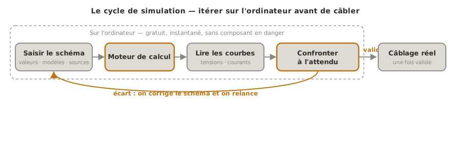
Whatever the tool, a simulation always follows the same sequence.
- Draw the schematic. Place the parts, fill in their values and their models, add the sources (supply, signal generator). This is where the fidelity of the result is decided (see Pitfalls).
- Choose the analysis that suits the question (operating point / transient / frequency).
- Place the probes. Say what you want to watch — a voltage at a node, the current in a branch. You only read well what you explicitly asked to be plotted.
- Run, then read the curves or the values.
- Compare with what you expected. A simulation result is only worth something against an expected order of magnitude. That is the step that turns a pretty curve into usable information, and it is covered just below.
Interpreting the results
This is half the work, and the half most often skipped: a simulation that runs tells you nothing until you have read what it shows. Three moves.
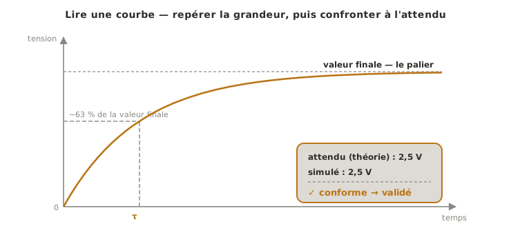
Read the quantity. Identify the axis, the unit and the scale before anything else: a curve “going up” means nothing until you know whether it tops out at 3.3 V or at 30 V, in 1 ms or in 1 s. Note the key values — maximum, resting value, rise time, cut-off frequency.
Compare with what you expected. Compare the result with what theory, the datasheet or the requirements predict. A 10 kΩ / 10 kΩ voltage divider on 5 V must give 2.5 V at its midpoint: if the simulation shows 2.5 V, it confirms what you entered. If it shows 5 V, then a wire is missing or a load is dragging the node down. A simulation is checked first on a case whose answer you already know.
Decide. Three outcomes are possible. The design is confirmed (you move on to building it). It needs revising (a value does not work, you iterate). Or the result is nonsense, and a nonsense result almost always means an error in what you entered or in a model, not a discovery about physics. The reflex in front of the implausible is not to believe it, but to re-read the schematic.
Choosing a simulator
Simulators fall into two families depending on what you are simulating: analog electronics (discrete parts, continuous signals) or microcontroller boards (where the code drives the circuit). The choice depends on the nature of the sub-assembly you are studying, and nothing stops you using both in the same project.
| Tool | Family | What stands out | When to use it |
|---|---|---|---|
| Falstad | analog | browser-based, no account, shows the current flowing | understanding and exploring fast, teaching |
| LTspice | analog (SPICE) | free (Analog Devices), complete and accurate analyses | serious sizing, power supplies, filters |
| Wokwi | microcontroller | browser-based, ESP32/Arduino/Pico + sensors, runs the code (C++ or MicroPython) | checking an MCU circuit plus code before the hardware |
| Tinkercad | microcontroller | Arduino sandbox plus simple electronics, online | first steps, beginner prototyping |
Two pointers to find your way. For analog work — a voltage divider, a filter, a power stage — stay with Falstad (to understand) or LTspice (to size). For a microcontroller circuit whose behaviour depends on the program, take Wokwi or Tinkercad, which run the code alongside the circuit.
Note
Simulating is not drawing. Tools like Fritzing are there to represent a circuit (breadboard view, schematic view, export towards the PCB), not to simulate how it behaves. They answer “what does my wiring look like?”, not “what does my circuit do?“. Not to be confused with the simulators above.
Pitfalls
Taking the simulation for reality. The simulator works on ideal models: unless you tell it otherwise, it ignores part tolerances, parasitic resistances, heating and noise. “It works in simulation” means “the logic of the circuit is right”, not “it will work on the bench”.
Garbage in, garbage out. A wrong value or a bad part model produces a result that is wrong but credible. Simulation does not correct an entry error, it propagates it neatly. Which is why you check on a known case first.
Running the wrong analysis. Looking for a bandwidth with a transient analysis, or a steady state with a frequency sweep, gets you an answer to the wrong question. The analysis follows from the question.
Not comparing. A curve with no expected order of magnitude is just a drawing. Always ask yourself “what value should I be finding?” before you run, so that you have a yardstick when you read.
Over-modelling something trivial. Bringing out LTspice and its full SPICE models to check that an LED lights up wastes more time than doing the sum in your head. The tool follows the need: Falstad to understand, SPICE to size things finely.
Where it fits in the project
- Concept phase — simulation helps you explore and freeze an electronic architecture: comparing two power stages, checking that a supply holds up under load, before settling it in a decision matrix.
- Proof of concept phase — simulate a sub-assembly before wiring it or ordering the parts: a few minutes that save a board you would have had to redo, or a burnt part.
- Towards real measurement — the simulated curve is the expected result you will then compare with the oscilloscope trace on the real circuit. Ideal simulation, normative datasheet, real measurement: three faces of one signal (see timing diagram).
See also
- Reading a schematic — reading the static diagram that simulation brings to life (prerequisite)
- Reading a datasheet — where the values and models you enter come from
- Timing diagram — reading a waveform, ideal or real
- Logic levels — simulation helps check level compatibility before wiring
- Falstad · LTspice — analog simulators (tool pages)
- Wokwi · Tinkercad — microcontroller board simulators (tool pages)
- Measuring instruments — the real counterpart: measuring on the bench what simulation predicted