A timing diagram is a graphical representation of how one or several signals evolve over time, drawn on a shared time axis. Where the other representations of an algorithm describe the logic (the chain of decisions or of states), the timing diagram describes the timing: it is there to check the timing relationships between signals — what changes before what, how long a pulse lasts, which edge to react to.
What is it for?
Plenty of embedded problems are not problems of logic but of time: does one signal have to rise before the other? how long does a pulse last? at what frequency? A timing diagram makes those questions visible. It is there to:
- read the timing diagrams in a datasheet — most components specify their signals in that form (see reading a datasheet);
- specify or check a protocol — the order and the duration of the bits in a UART, I²C or SPI frame;
- characterise a PWM signal — period, high time, duty cycle;
- set the expected against the real — the ideal diagram is compared with what the oscilloscope shows on the actual build.
It is the representation to reach for as soon as a timing constraint comes into play, alongside the others: you describe what to do with a state machine, and when with a timing diagram.
A status of its own. The timing diagram is not a fourth way of describing the logic: it is the only one of the four representations that talks about the hardware. Flowchart, state machine and GRAFCET handle abstractions — decisions, states, steps — and turn into code. The timing diagram shows physical quantities, voltages switching over time. It is also the only one you can measure on the real system (oscilloscope, logic analyser). And the further down you go towards the low level — the bits of a bus, the timings in a datasheet, PWM — the more the question stops being “what logic?” and becomes “when, exactly?”: that is where it becomes the main tool.
How to read a timing diagram
Everything is read against the horizontal time axis, shared by every signal and running to the right.
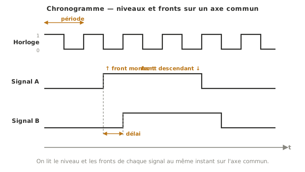
- Levels. A logic signal only takes two levels: high (1) and low (0). The line stays at one level, then switches.
- Edges. The move 0 → 1 is a rising edge (↑), the move 1 → 0 a falling edge (↓). It is often on an edge, not on a level, that an action is triggered.
- Durations. You read the period T (the pattern that repeats), the high time tₕ, and for a PWM signal the duty cycle α = tₕ / T. The subscript is the French haut, that is high. The notation is kept as it appears on the diagrams.
- Vertical alignment means simultaneity. Whatever sits at the same horizontal position happens at the same instant. A dashed vertical line is used to read a relationship: an edge on A brings about a change on B after a certain delay.
The reading rule fits in one sentence: you pick an instant on the axis, and you read the level of every signal at that instant.
Example — PWM signal and serial frame
Two signals you meet constantly on a project, read on the same axis.
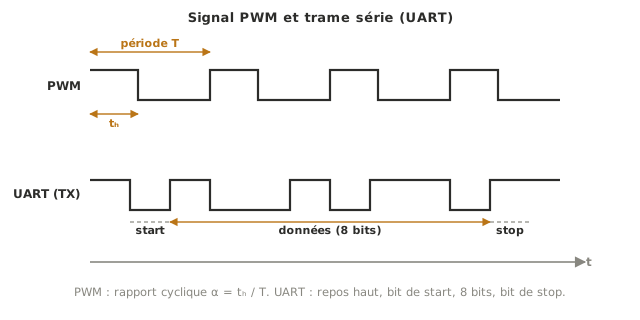
The PWM signal (top) is a square wave where only the duty cycle α = tₕ / T matters: at a fixed frequency, the longer the high time, the greater the average power delivered (motor speed, LED brightness: see driving a PWM output). The UART frame (bottom) shows the other use: the line sits high at rest, a start bit (low) announces the frame, then come the 8 data bits, then a stop bit. Without a timing diagram, there is no way to check that each bit is sampled at the right instant.
Pitfalls
No shared time axis. Drawing each signal on its own scale makes any reading of a relationship impossible. Every signal shares the same horizontal axis, or the diagram means nothing.
Mixing up level and edge. Reacting “while it is high” and reacting “on the rising edge” are two different things. Plenty of bugs (button bounce, double counts) come from that confusion.
No time scale. With no scale marks and no reference duration, you can see the order of events but you cannot measure anything. Give at least one duration or one period.
Mixing up logic and analog. A logic timing diagram has only two levels. A signal that varies continuously (a sensor voltage) is a curve. Drawing it belongs to the oscilloscope instead.
Mixing up duty cycle and frequency. The duty cycle (α = tₕ/T) says what fraction of the time the signal is high. The frequency (1/T) says how often it repeats. You can change one without the other.
Reading relationships without aligning. Judging that “A changes before B” without drawing the vertical line in the right place leads to mistakes about what causes what. Align vertically before concluding.
Special case — From the timing diagram to the oscilloscope
The timing diagram exists in three complementary forms. Idealised, it is a design tool (perfect signals, vertical edges). Normative, it is the timing diagram in a datasheet, which fixes the minimum durations to respect. Real, it is what the oscilloscope draws on the build, or what a logic analyser captures across several lines at once, with all its imperfections (a rise time that is not zero, noise, bounce). Being able to read an ideal diagram is the prerequisite for interpreting the other two.
See also
- Algorithm — the parent page, where the timing diagram is the representation of time
- Oscilloscope — the instrument that displays a signal’s real timing diagram
- Logic analyser — the real timing diagram of several digital lines, with frames decoded
- Reading a datasheet — where you meet the normative timing diagrams of components
- Driving a PWM output (Arduino) — generating a signal whose duty cycle reads off a timing diagram
- Driving a PWM output (MicroPython) — the same signal, on the MicroPython side
- UART — the serial frame whose timing diagram fixes the order of the bits