Falstad

Falstad (named after its author, Paul Falstad — Circuit Simulator, at falstad.com/circuit) is a simulator for analog circuits that runs in the browser, free and with no account. Its signature: it shows the current flowing as moving dots, and voltage through a colour code. It is the tool for understanding a circuit and exploring it fast — less so for sizing it precisely (see LTspice). This page is a tool tutorial belonging to the circuit simulation hub, which carries the general method. What you learn here are the moves, in three steps: read a running circuit, modify one, then build one. Best followed with the screen in front of you. Falstad follows your browser’s language, and the screenshots here were taken with the interface in French: menu names are quoted as they appear in the pictures, with a plain English rendering in brackets at first use, and an English interface puts the same entries in the same places.

What is it for?

You open it to:

• see what a schematic does — the current speeding up in a branch when you lower its resistance, a voltage collapsing under too heavy a load;
• explore in real time — change a value and watch the effect straight away, with nothing to re-run;
• start with nothing to install — no software, no account, which makes it ideal in class or for a first attempt.

The trade-off: its parts are ideal and generic. To confirm a sizing, you move on to LTspice.

Reading a running circuit

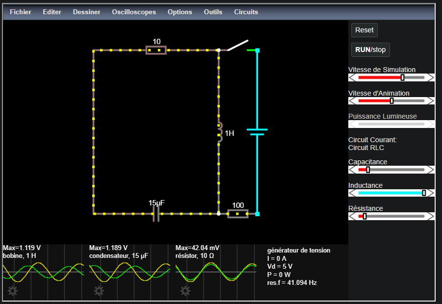
The page opens on a circuit that is already running — an RLC circuit, with its three scopes already placed at the bottom of the window. Before touching anything at all, you have to be able to read the screen: that is where Falstad gives the most.

• Colour is voltage: green for a positive voltage, grey for the reference potential, red for a negative voltage, the shade following the amplitude. A wire turning red is not faulty, it is at a negative voltage.
• The dots are the current: they move in the conventional direction, and their speed is proportional to the current. A branch where the dots crawl conducts little. A frozen branch does not conduct at all.
• Hovering is measuring: pointing at a part fills the panel at the bottom right. You read there its nature, the current I through it, the voltage Vd across it, its value and the power P it dissipates. It is Falstad’s multimeter, with no probe to wire.

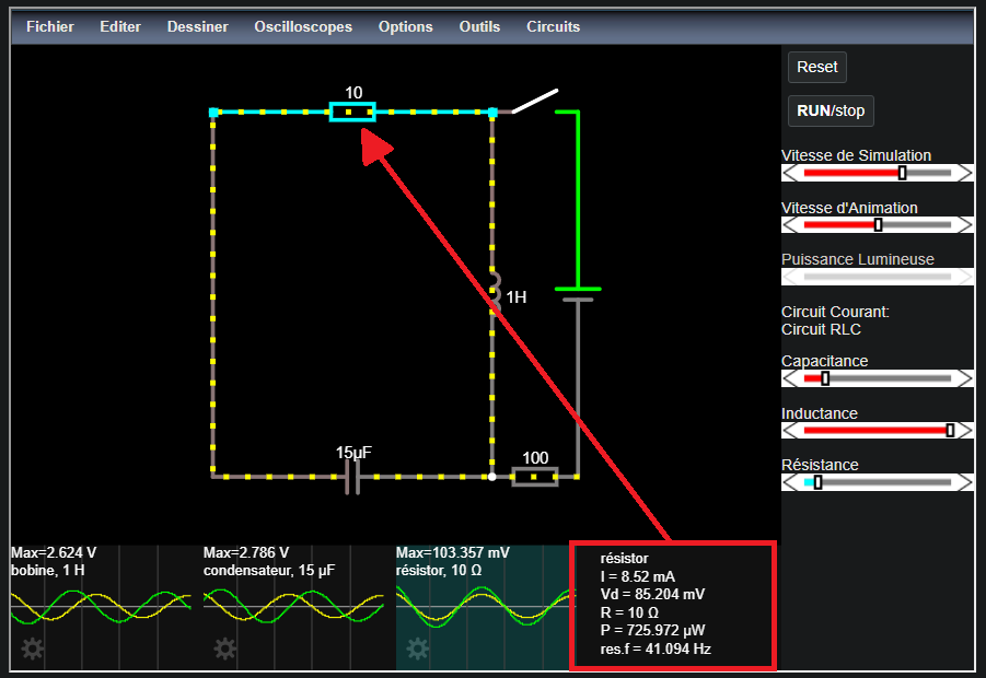
Hovering also highlights the scope belonging to the part you point at: it is the shortest bridge between the schematic and the curve, and it is worth making a reflex of it.

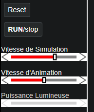
The simulation runs continuously. RUN/stop freezes and restarts it, Reset starts over from zero. Three sliders follow in the right-hand column, and the first two are regularly confused with each other.

Warning

Vitesse de Simulation and Vitesse d’Animation (Simulation Speed and Animation Speed) do not do the same thing. Vitesse de Simulation sets the flow of simulated time. That is the one you adjust to watch a fast phenomenon, and it has no effect at all on a purely resistive circuit. Vitesse d’Animation only sets the speed of the dots: visual comfort, with no influence on the measured values. Slowing the dots down while believing you are slowing time down, then drawing a conclusion about a duration, is the most frequent reading error with this tool. The third slider, Puissance Lumineuse (Power Brightness), only affects the brightness of the display.

Modifying an existing circuit

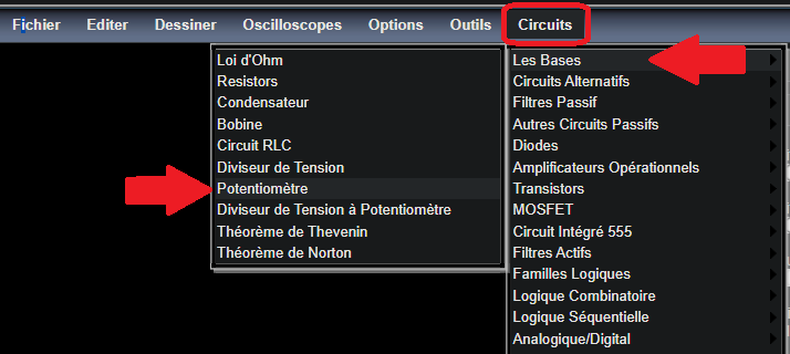
The Circuits menu holds a well-stocked library, arranged by theme — Les Bases (Basics), Circuits Alternatifs (AC circuits), Filtres Passif (passive filters), diodes, operational amplifiers, logic. Starting from one of these circuits and transforming it is the most profitable move the tool offers: the circuit is already correct, so attention is spent only on what you change.

1. Load the circuit and edit it

Open Circuits → Les Bases → Potentiomètre (Circuits → Basics → Potentiometer).

The circuit is a peculiar one, and it has to be read before being touched: two 5 V sources have their + terminal tied to the wiper of the potentiometer, and each has its − terminal tied to one end of the track. Each half-track therefore has the whole 5 V across it, and forms its own loop with its own source.

A double-click on a part opens its settings. That is the central editing move in Falstad. On the potentiometer, the box announces a total resistance of 1 kΩ, and the schematic shows 500 and 500 on either side of the wiper: the two halves are equal.

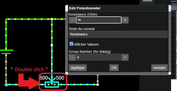
The potentiometer also gets a setting slider in the right-hand column. Its label is the Texte du curseur (Slider Text) field of the edit box. The mouse wheel, with the pointer on the part, does the same thing. And to remove an element rather than modify it, select it and press Suppr (Delete).

Question

Predict before you sweep. Each half-track sees 5 V across it, and moving the wiper redistributes the 1 kΩ between the two halves. Pushing the wiper towards one end: will the two currents simply swap, or will one of them run away? Write your answer down before moving anything.

2. Sweep and watch

At mid-travel, each half is 500 Ω and carries 5 V: 10 mA on each side, 20 mA in all. Pushed to a tenth of its travel, the ratio blows up. 100 Ω on one side let 50 mA through, the 900 Ω on the other let only 5.6 mA through, nine times less. The dots race away in one branch while they grind to a halt in the other.

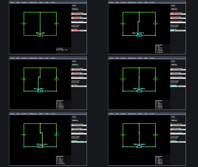
This is Ohm’s law made visible: at constant voltage, current is the inverse of resistance. A formula recited for years becomes, in a few seconds of sweeping, something you have seen.

Note

This circuit is a demonstration, not a project circuit. Nobody wires two supplies onto the wiper of a potentiometer. In a project, the potentiometer serves as a voltage divider — the whole track between supply and ground, the voltage taken off the wiper and read by an analog-to-digital converter: that is the Diviseur de Tension à Potentiomètre (Voltage Divider with Potentiometer) entry in the same menu, and it is the circuit described on the The potentiometer page.

Building your own circuit — A high-pass filter

That leaves the complete move: starting from nothing. We build an RC high-pass filter, and watch what it lets through depending on frequency.

1. Blank page and placing parts

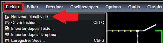
Fichier → Nouveau circuit vide (File → New Blank Circuit) empties the drawing area. Careful: a circuit with no voltage source will not start.

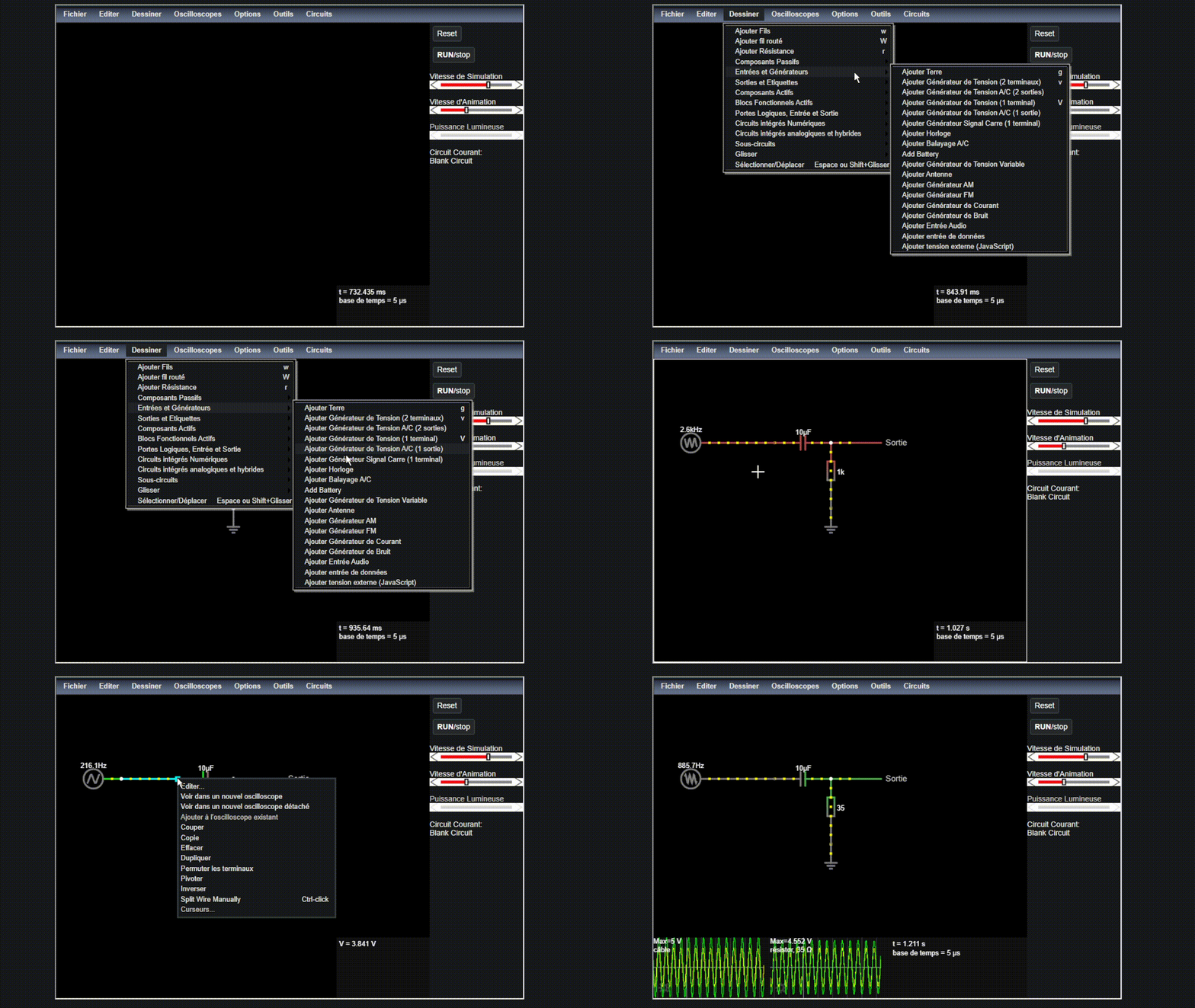
Everything is placed from the Dessiner (Draw) menu, which carries the whole catalogue. Three entries sit directly at the top level, because they are the most used:

• Ajouter fils (Add Wire, w) — the straight wire, the one you use all the time;
• Ajouter fils routé (Add Routed Wire, W) — the variant that finds its way round on its own;
• Ajouter résistance (Add Resistor, r).

The rest is filed in submenus: Composants passifs (passive components: capacitor, inductor, potentiometer), Entrées et générateurs (inputs and sources: DC and AC sources, signal generators, and ground), Sorties et étiquettes (outputs and labels), Composants actifs (active components: diodes, transistors, operational amplifiers), Blocs fonctionnels actifs (active building blocks), then the whole digital part (Portes logiques, Circuits intégrés numériques, Circuits intégrés analogiques et hybrides, that is logic gates, digital chips, analog and hybrid chips) and the Sous-circuits (subcircuits).

The move is the same for all of them: you pick the type in the menu, the pointer turns into a cross, and you draw the part by clicking and dragging from one terminal to the other. Two last entries of the menu place nothing but change mode — Glisser and Sélectionner/déplacer (drag, and select/move, with Space, or Shift + drag): that is how you get the normal pointer back, which unblocks many a situation where the tool seems stuck placing parts for ever.

What is needed here is a 5 V AC voltage source (Entrées et générateurs), a 10 µF capacitor in series (Composants passifs), a 35 Ω resistor towards ground (r, at the top level) and ground itself — Entrées et générateurs → Ajouter terre (Add Ground), shortcut g. It is the reference potential all displayed voltages are referred to, and the grey of the colour code. The output is read across the resistor: that is what makes this a high-pass rather than a low-pass filter.

Note

The menu says “earth”, we say “ground”. The symbol that Ajouter terre places is the one for ground — the 0 V reference node of the circuit. In electrical work, “earth” means something else: the protective connection to the soil, the one on the third wire of a mains socket. It is a shortcut in the software’s French wording (English ground covers both), and not one to take up in a report.

Warning

Falstad will not stop you. Short a 5 V source out with a plain wire: no message, no alert, the simulation carries on, and hovering calmly announces I = 5 kA. Five thousand amps. The figure is not a glitch: in the model, a “perfect” wire is worth about 1 mΩ, and 5 V across 1 mΩ makes exactly 5 000 A. On a bench, that same circuit destroys the supply in a fraction of a second. This is the most important limit of the tool: it computes what you ask it for, it does not judge whether that is buildable. An absurd current value is not a discovery, it is a signal.

2. Predict, then sweep the frequency

Place one scope on the input and one on the output (the Oscilloscopes menu and right-clicking a part both handle them), then vary the frequency of the source.

Question

Predict before you sweep. The cut-off frequency of an RC filter is fc = 1 / (2π·R·C). With 35 Ω and 10 µF, where does it fall? And for a high-pass, will the output be larger at 20 Hz or at 1 kHz?

3. Read and compare

Theory gives fc = 1 / (2π × 35 Ω × 10 µF) ≈ 455 Hz, right in the middle of the swept range. Below it, the filter cuts. Above it, it lets through.

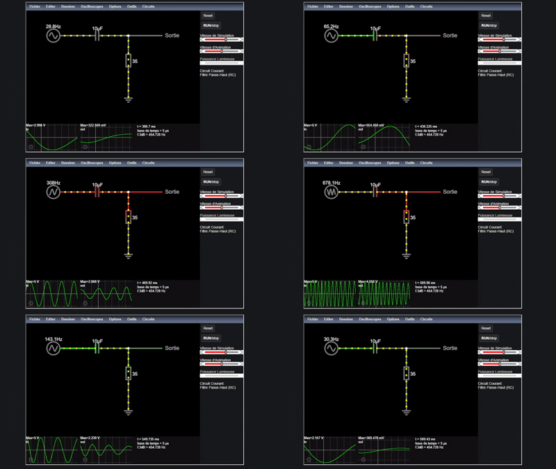
At 20 Hz, the output does not exceed a few hundred millivolts — some twenty times less than the input: the filter cuts. At 1 kHz, it reaches 4.55 V, or 91% of the input: the filter lets through. That last point is the one to compare, because theory predicts it exactly: at f = 2.2 × fc, a first-order high-pass gives back a gain of 0.91. The simulation does not merely “draw a nice curve”, it lands on the expected value, and it is that comparison, not the curve, that validates what you entered.

If the deformation scrolls past too fast to be read, it is Vitesse de Simulation that has to be slowed down, and not Vitesse d’Animation, which will only drag the dots along a curve that is just as unreadable.

4. Keeping the circuit

Tip

With no account, exporting is the real save. The Fichier menu offers Exporter comme Texte… (Export As Text, a file to keep in the project folder) and Exporter avec Lien… (Export As Url), which encodes the whole circuit in a URL: that is how you send a circuit to a classmate or a supervisor, with nothing for them to install. For a report, Exporter en SVG… and Exporter comme Image… (Export As SVG and Export As Image) put the schematic out cleanly.

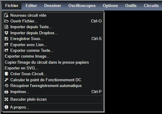
We have just checked a cut-off frequency on a curve, and the temptation is immediate: to believe the filter is sized. It is not. Falstad simulates in the time domain and lets you change the frequency by hand, but it plots no frequency response. The day you have to read a cut-off at the −3 dB point on an automatic sweep, or to account for real parts, LTspice is what you open.

Importing a circuit written as text

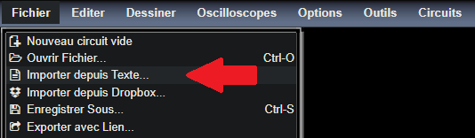
The three previous sections all start from a move on screen. There is a fourth way in, more unexpected: a Falstad circuit is a text file, and the tool knows how to read one back. Fichier → Importer depuis Texte… (Import From Text) opens a box where you paste the description of a circuit you have not drawn.

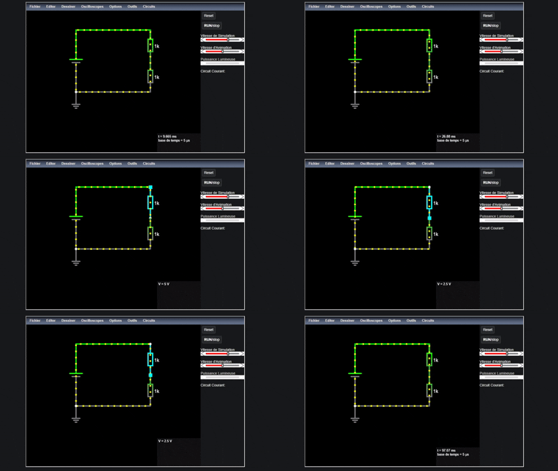
Here is the description of a voltage divider: a 5 V DC source and two 1 kΩ resistors in series.

$ 1 0.000005 10.20027730826997 50 5 43 5e-11
v 176 336 176 176 0 0 40 5 0 0 0.5
w 176 176 368 176 0
r 368 176 368 256 0 1000
r 368 256 368 336 0 1000
w 368 336 176 336 0
g 176 336 176 368 0

Each line is a part: its letter (v voltage source, r resistor, w wire, g ground), the coordinates of its two terminals, then its values — 5 volts for the source, 1000 ohms for each resistor. The first line, the one beginning with $, describes no part at all: it carries the simulation settings. Two parts are connected as soon as they share coordinates, and the two resistors meet at point 368 256, which becomes the midpoint of the divider.

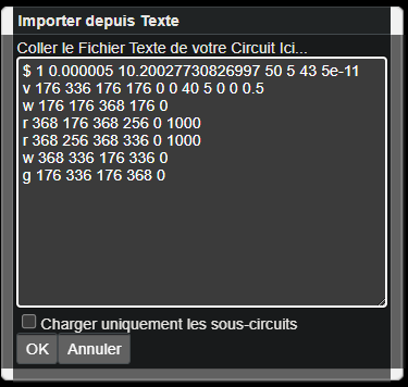
One click on OK and the circuit appears, powered up. What remains is to check that it does what you expected: at the top of the divider, hovering gives the 5 V of the source, and 2.5 V at the midpoint, half of it, since the two resistors are equal.

Tip

Have a circuit described, then check it yourself. The description above was produced by an artificial intelligence asked for a divide-by-two voltage divider. It is an interesting use, provided you see clearly where the work lies: what is produced is not an answer, it is a hypothesis, and Falstad puts it under power to make it checkable. Does the current go where you expect it? Does the voltage at the midpoint match what the sum says? A wrong circuit imports just as well as a right one: it is the simulation, and your reading of the result, that settle it. Used that way, the trick saves the time of the drawing and gives it back to the reasoning.

The criterion holds beyond this case, and in both directions: is the statement produced checkable on screen? A proposed circuit can be powered up, an announced voltage can be read by hovering. Those are hypotheses. A sizing conclusion, on the other hand, cannot be checked: it has to be produced, and that is the work that cannot be delegated. Same rule over on the LTspice side, where what you hand over to be read is a netlist.

Two limits worth knowing. The format also encodes the positions on screen, so a generated circuit can be electrically correct and graphically crooked. Coordinates snap to a grid, and an approximate text produces an unreadable schematic. And this is not a netlist in the board-design sense: a netlist describes only the connections between pins, with no geometry, and that is the one you will meet when moving from the schematic to the printed circuit board.

Pitfalls

Taking an ideal model for reality. Falstad’s parts have no tolerance, no parasitic resistance and no heating, and nothing warns you that a current is destructive (see the 5 kA short above): the tool gives the right behaviour, not the guaranteed value of a real part, and the general pitfalls of simulation apply here too.

Confusing the two speeds. Vitesse d’Animation only affects the speed of the dots. Only Vitesse de Simulation changes the flow of simulated time. Concluding about a duration after touching the wrong slider gives a wrong answer on a screen that seems to have obeyed.

Relying on the auto-save. Fichier → Récupérer l’enregistrement automatique (Recover Auto-Save) does exist and does sometimes save the day, but it is a safety net, not a save: it keeps one state only, and it does not survive a change of machine. Export as soon as a circuit is worth keeping.

Taking a demonstration circuit for a project circuit. The library is built to show a phenomenon, not to be copied onto a board. Before transposing, ask yourself whether the wiring makes sense outside the simulator.

Exercises

Question

Exercise 1 — Moving the cut-off. Take the high-pass filter again and replace the 35 Ω resistor with 350 Ω. Before re-running: where does the new cut-off frequency fall? And what becomes of the output at 20 Hz — larger or smaller than before? Then check on screen.

Solution

fc = 1 / (2π × 350 Ω × 10 µF) ≈ 45.5 Hz, ten times lower: multiplying R by ten divides the cut-off by ten. At 20 Hz you are no longer far below the cut-off, and the output rises to about 2 V instead of 0.3 V. The filter cuts less low, so it lets more of the low frequencies through, which is indeed the behaviour expected when you lower the cut-off of a high-pass.

Question

Exercise 2 — Making 3.3 V from 5 V. On a blank page, build a voltage divider that delivers 3.3 V from a 5 V DC source, using resistors of common values. Check the voltage by hovering, then say under what condition this circuit is usable in a real project.

Solution

A divider of 10 kΩ (source side) and 20 kΩ (ground side) gives 5 V × 20 / (10 + 20) = 3.33 V, and draws 5 V / 30 kΩ ≈ 0.17 mA.

The condition lies in that current: the circuit is only worth anything if it drives a high-impedance input (that of an analog-to-digital converter, for instance) which draws next to nothing. As soon as a load draws current at the midpoint, it sits in parallel with the lower resistor and pulls the voltage down. A divider never supplies a part. See logic levels.

See also

• Circuit simulation — the hub: method, types of analysis and reading of results
• LTspice — the tool for precise sizing, when the values matter
• The potentiometer — the part from section 2, in its project wiring
• Timing diagram — reading a waveform, ideal or real
• Logic levels — why a divider does not replace a supply
• Reading a schematic — the schematic that Falstad brings to life