LTspice

LTspice (published free of charge by Analog Devices) is the reference SPICE simulator for the precise sizing of an analog circuit. Where Falstad makes you understand, LTspice makes you decide: real part models, complete analyses, faithful results. It is the tool the Falstad page announces at its close, the one you open the day you have to read off a cut-off frequency at the −3 dB point instead of guessing it by changing the frequency by hand. This page is a tool tutorial belonging to the circuit simulation hub, which carries the general method. What you learn here are the moves, in the same order as on Falstad — read a running circuit, modify one, then build one — preceded by a step Falstad did without: installing. Best followed with the screen in front of you.

Note

LTspice is not localised. The menus read File, Simulate, View whatever the machine and whatever the language it is set to. It is worth knowing, because it means the wording quoted here is the wording you will meet again in the Analog Devices documentation and in just about every tutorial you go on to find.

What is it for?

You open it to:

• size things seriously — pick a part value knowing the real margin, not an order of magnitude;
• sweep a whole range in one go — ask for the gain over five decades and read the cut-off off with a cursor, where a real-time simulator forces you to change the frequency by hand;
• simulate parts that exist. The built-in catalogue holds the Analog Devices references, and a Contrib folder gathers those of other manufacturers.
• produce quotable values for a technical design file: a cut-off read off a curve, not eyeballed.

The trade-off: nothing is animated, nothing recomputes on its own, and nothing appears at all until a directive has said which question you are asking. To explore fast and watch the current flow, you stay on Falstad.

Installing LTspice

This is the one step Falstad did not impose, and it takes a few minutes.

The software is downloaded from the Analog Devices site. It is free, with no account, no key and no limit on circuit size, and there is no crippled version you would have to grow out of later. Two systems are served: Windows and macOS.

Warning

There is no Linux build. That is a hardware constraint, not a setting: on a Linux machine you have to plan another way round (a school machine, a workstation shared with a partner) or stay on Falstad for the exploration part. Better to find that out at the start of a project than the evening before a review.

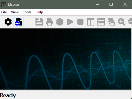
At first launch the window is empty: no welcome circuit, no animation, and most buttons greyed out. That is normal, and it is the first thing that throws you when you arrive from Falstad.

You are not starting from nothing, though. The tool ships with a library of examples, and that is where you begin.

Reading a circuit that already runs

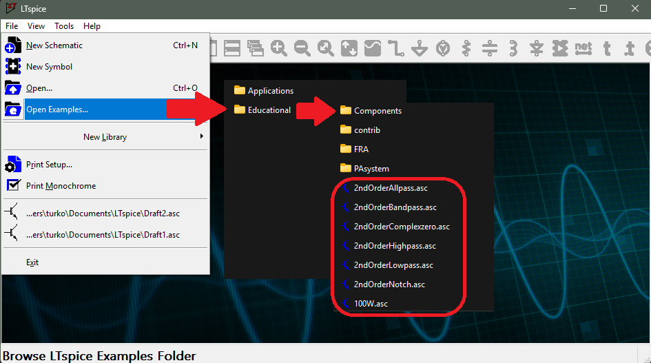
File → Open Examples…, then the Educational folder: the entry opens a cascade of menus that unfolds the tree of examples directly, without going through a dialog box. The .asc files you find there already carry their simulation directive: they run as they are, with nothing to edit. Opening one and running the simulation gives you, in two clicks, the screen you have to learn to read.

Three things are to be read, and they are not in the same place.

• The schematic — the parts and their values, as on any schematic. Nothing moves on it: no colour signals a voltage, no dot embodies a current.
• The directive — a line of text placed on the schematic, of the kind .tran 5m or .ac dec 100 10 100k. It is what says which analysis was asked for, and it is the element Falstad does not have at all. Reading it first saves a lot of misunderstandings: it announces in advance what the curve can and cannot show.
• The plot — the waveform window, with its horizontal axis in time or in frequency depending on the directive, and its traces named after the node, V(out) or I(R1).

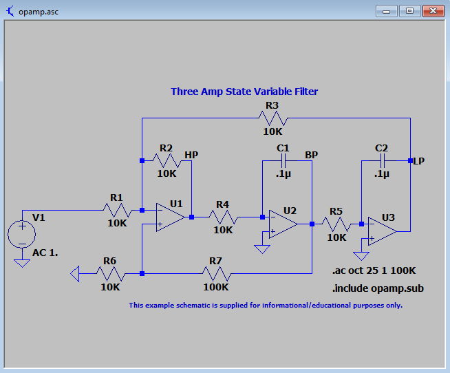
On this example, the .ac oct 25 1 100K directive is placed on the schematic like any other text: it asks for a sweep from 1 Hz to 100 kHz, by octaves, at 25 points per octave. The AC 1. mention under the source says, for its part, that the input amplitude of the sweep is 1. Those are two pieces of information no paper schematic carries, and without which the curve means nothing.

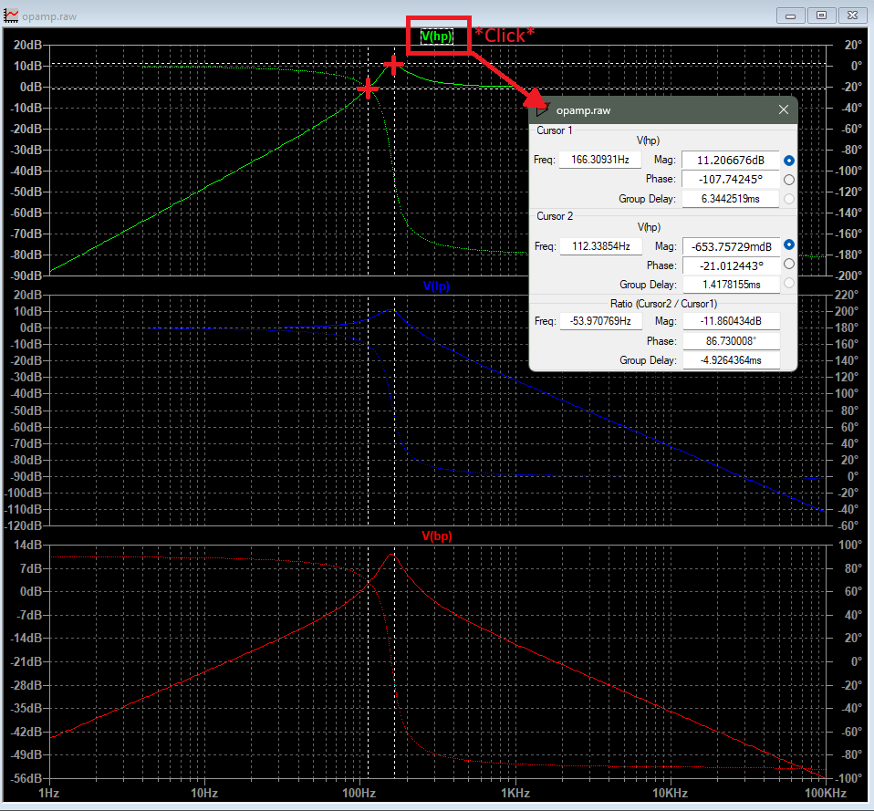
The measuring move takes one click: click the label of a trace, at the top of the graph. A cursor latches onto the curve and a readout window opens. On a frequency analysis it gives, for the point aimed at, the frequency (Freq), the gain in decibels (Mag) and the phase (Phase). On a transient analysis, the abscissa is a time. A double-click on that same label places two cursors: the window then shows both positions and, below them, their ratio (Ratio). That is what you want as soon as a reading calls for two — reading an overshoot at one place and the phase at another, measuring a duration, comparing two gains.

Note

What you hover over on one side you click on the other. On Falstad, pointing at a part is enough to read its current and its voltage, live and with nothing to launch. Here you first have to have simulated, then designate a trace. It is the first sign of a difference of principle: Falstad computes all the time, LTspice computes on demand.

Modifying an existing circuit

The circuit from the library is already correct, so attention is spent only on what you change. This is the moment to learn the central move of the tool, on a circuit you have no reason to doubt.

1. Ask the same circuit a different question

The directive is not a technical setting, it is the question. Five of them are enough on a project, and three cover the essentials (see the table of the three families of analysis on the hub):

• .op — the operating point: voltages and currents at rest, one value per node, no curve (DC op pnt tab);
• .tran — transient analysis: evolution over time, horizontal axis in seconds (Transient tab);
• .ac — frequency analysis: gain and phase over a range of frequencies, horizontal axis in hertz (AC Analysis tab).

Two more turn up quickly: .dc (sweeping a DC source, to trace the characteristic of a diode or a transistor) and .noise (noise). One and the same directive can be written by hand on the schematic, or set in the tabbed dialog opened by Simulate → Configure Analysis (shortcut A): you fill the fields in, the dialog composes the command line and places it on the schematic. The bottom of the dialog recalls the expected syntax and shows the directive it has built. That is the best place to learn to write them yourself.

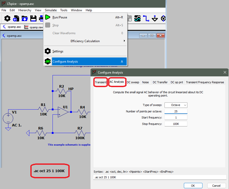
2. Switch from one analysis to another

The shortcut that makes this spectacular: Shift + left-click on a text on the schematic toggles it between directive and comment. Comment the existing directive out, write (or uncomment) another one, re-run. The same circuit answers a different question, and the plot window changes axis. The two directives can live side by side on the schematic, as long as only one is active at a time.

Question

Predict before you switch. The circuit does not change one bit, only the directive changes. Before re-running: will the horizontal axis stay the same? Will the curve still show what happens at an instant, or what happens at a frequency? And if the new window came out empty, what would you have to put that down to?

3. Change a value — and remember to re-run

A right-click on a part opens its settings. You enter a new value and confirm. And the curve on screen does not move: it is still the one from the previous run. You have to re-run with the ▶ button (Simulate → Run/Pause, Alt+R).

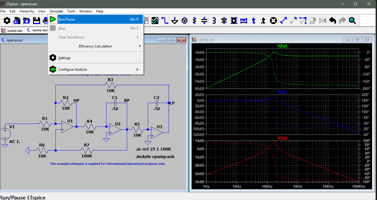
This is the most frequent mistake when arriving from Falstad, where every change was reflected on screen immediately. Here, a plot is never more than a photograph of the last computation, and nothing tells you it has aged.

Building your own circuit — A low-pass filter

That leaves the complete move: starting from nothing. We build an RC low-pass filter and read off its cut-off frequency, the measurement Falstad cannot produce.

1. Blank page and placing parts

File → New Schematic (Ctrl+N) opens a blank sheet. The most common parts — resistor, capacitor, wire, ground — have their button in the toolbar and their keyboard shortcut. Everything else, sources included, is picked from the catalogue through Edit → Component. To identify a button, just hover over it: its name and its shortcut appear in the status bar, at the bottom of the window.

What is needed here is a voltage source, a 1 kΩ resistor in series, a 160 nF capacitor towards ground, and ground itself. The circuit is a single mesh: the source feeds the resistor, the resistor feeds the capacitor, the capacitor comes back down to ground. The output is read across the capacitor, and that is what makes this a low-pass rather than a high-pass filter.

Warning

With no ground, nothing simulates. SPICE needs a 0 V reference node to refer every voltage to. A schematic with no ground fails, with a message that does not frankly say why. It is beginner mistake number one under SPICE, and it does not forgive: it blocks everything, whatever the directive.

One last move, and it will pay off twice: label the nodes. Placing an in label at the input and an out label on the output makes the traces appear under the names V(in) and V(out) instead of V(n001) and V(n002). The plot becomes readable at a glance, and so does the text description of the circuit, which will be useful further on.

2. Set the source up for the frequency sweep

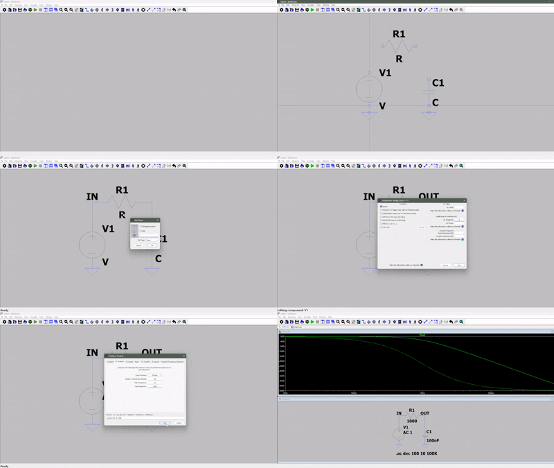
A voltage source carries several independent settings, and that is where the trap of frequency analysis lies. Right-clicking the source, then the Advanced button, opens the full dialog: there you find the DC value, the time-domain waveform (SINE, PULSE…), and, in a section of its own, the amplitude for small-signal analysis, the one .ac uses. That is the field to fill in, at 1: the gain will then read directly as a ratio to the input. Going through this dialog can be seen in the video sequence at the end of this section.

Warning

A source with no AC amplitude gives an empty curve. The amplitude of the time-domain waveform and the small-signal amplitude are two different fields. Filling the first in and running an .ac produces a flat plot, a null one, or a window in which there seems to be nothing at all — without the slightest error message. Faced with an .ac that “shows nothing”, that is the first thing to check, before even suspecting the circuit.

3. Place the directive and predict

The sweep directive is written .ac dec 100 10 100k: sweep by decades, 100 points per decade, from 10 Hz to 100 kHz. Five decades, plenty to bracket the expected cut-off. In the Configure Analysis dialog, AC Analysis tab, this amounts to choosing Decade as the sweep type and filling in the three following fields. The line composes itself at the bottom of the dialog.

Question

Predict before you run. The cut-off frequency of an RC filter is fc = 1 / (2π·R·C). With 1 kΩ and 160 nF, where does it fall? And by how many decibels will the gain have dropped at that precise frequency? Because that figure depends neither on R, nor on C, nor on the circuit you chose.

4. Read off the −3 dB point and compare

Theory gives fc = 1 / (2π × 1 kΩ × 160 nF) ≈ 995 Hz, and the gain there is exactly −3.01 dB. That is the very definition of the cut-off frequency, the point where the output voltage has fallen to 1/√2 of the input.

On the curve, the move is the one learned above: click the V(out) label, then bring the cursor along until the readout window shows about −3 dB. The frequency read off is the measured cut-off, and it should fall in the neighbourhood of 995 Hz.

It is that comparison, and not the curve, that validates what you entered: a clear gap between the 995 Hz calculated and the frequency read off does not say the filter is bad, it says a value was entered wrongly or a wire is missing. Once the two figures agree, the cut-off is a quotable value, and it can go as it stands into a sizing note.

The complete sequence, from blank sheet to cursor sitting on the −3 dB point, takes a little over a minute. To be watched after trying, so as to compare the moves, not before, on pain of copying instead of building.

Note

The same circuit, known in two ways. On Falstad you would have changed the frequency of the source by hand and watched the output sine shrink: you feel the filter working, but you read off no cut-off, because the tool simulates in the time domain and plots no frequency response. LTspice shows nothing of the current flowing, but it sweeps five decades and gives you the figure at the cursor. One gives the intuition, the other the value. A serious project goes through both, and in that order.

Tip

Parts that exist, with nothing more to install. The Edit → Component catalogue does not hold only ideal parts: you find the Analog Devices references there and, in the Contrib folder, those of other manufacturers. A button in it even opens an example circuit for the selected reference — often the typical circuit from its datasheet. A model missing from the catalogue can be imported from a .lib or .mod file supplied by the manufacturer, but the real cost is not the import: it is the pairing of a symbol with the model, a detour that goes well beyond the scope of a project. Look in the catalogue first, or for an equivalent reference. And precision buys back nothing: an exact model on a wrongly entered value gives a result that is precise and wrong.

Exporting the netlist

An LTspice schematic has a text description, and the tool knows how to show it: View → Update and View SPICE Netlist opens a window where the circuit appears in a few lines — one part per line, its nodes, its value — followed by the directives placed on the schematic. The content can be selected and copied.

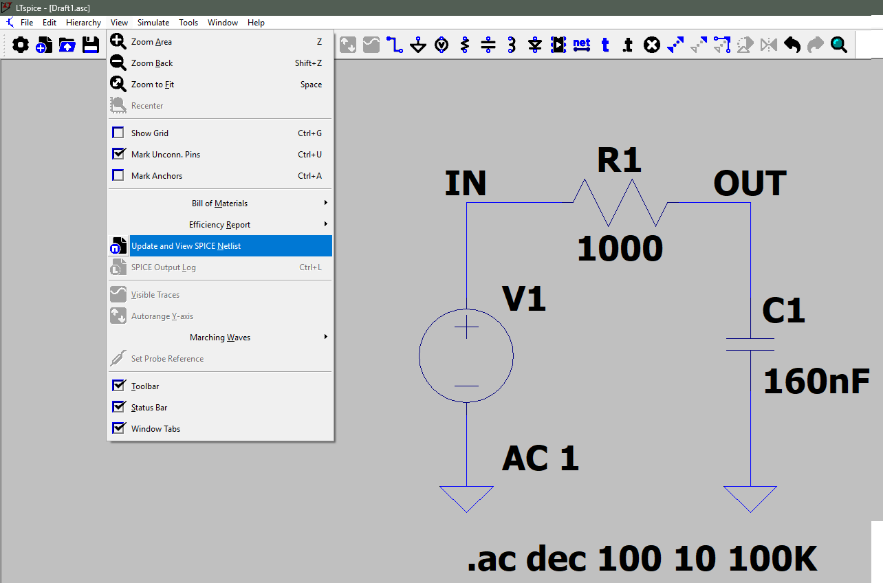
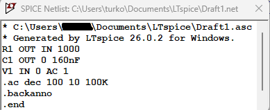
Four lines are enough to describe the filter: each part gives its name, the two nodes it is connected between, and its value. Ground carries the number 0. That is the SPICE convention, and it is why its absence blocks everything. The source shows its sweep amplitude after its nodes. And the directive is copied across as it stands from the schematic: the text therefore says both what the circuit is made of and what question it was asked.

This is where labelling the nodes pays off: without it, the netlist speaks in n001 and n002, and nobody knows which node is the output any more — not a classmate, not a supervisor, not you yourself three weeks later.

Warning

Two netlists, two uses. View → Update and View SPICE Netlist gives the electrical description, directives included: it appears on screen, it can be selected and copied. That is the one the simulator reads, and the one you share to have a circuit analysed. Tools → Export Netlist does something else: it writes a .net file to disk, meant for the routing of a board, the one you will meet when moving on to the printed circuit board, and it describes only the connections between pins, with no geometry and no analysis. For any use where the text has to be read back or pasted elsewhere, it is the first one you want, not the second.

Tip

Have a netlist read by an assistant, and keep the judgement. A netlist is a short text, with no geometry and no ambiguity: it pastes as it stands into a conversational assistant, which you can ask what the circuit does, or why a plot does not look like what you expected. The framing is the same as in Falstad, taken from the other end: what the assistant produces is not an answer, it is a hypothesis, and the criterion fits in one question, is this statement checkable on screen? “The AC amplitude of the source is at zero” is checked in three clicks. “The gain at 1 kHz is −3 dB” is checked with the cursor. Whereas “use 330 nF” is not a checkable hypothesis: it is the conclusion, and having it produced by a third party amounts to delegating the one piece of work that cannot be delegated.

One technical limit on top of that: the netlist does not carry the contents of external .lib files. On a circuit with a real part, the assistant does not know the model and will fill the gap in by itself.

Pitfalls

Forgetting to re-run. A changed value does not update the plot: the curve on screen is the one from the previous computation, and nothing signals it. A reflex to acquire: every change to the schematic ends with a Run/Pause.

Forgetting the ground. With no reference node, the simulation fails whatever the directive. The most frequent beginner mistake under SPICE, and the quickest to fix once identified.

Running the wrong directive. Looking for a cut-off frequency with .tran, or a steady state with .ac, gives a correct answer to a question you were not asking. The directive follows from the question, never the other way round.

Convergence failure. SPICE can refuse to converge on certain circuits — feedback loops, stiff models, fast switching. The message is disconcerting but the case is a classic: it is dealt with by adjusting the simulation options or simplifying the model, not by concluding that the circuit is wrong.

Over-tooling a trivial case. Checking that an LED lights up does not justify installing LTspice, entering a schematic in it and placing a directive: Falstad answers in thirty seconds. LTspice is kept for the cases where the exact value matters.

Exercises

Question

Exercise 1 — The wrong question. Take the low-pass filter again and, instead of the .ac, run a .tran 10m transient analysis with a sine source at 1 kHz. Describe what the resulting curve shows, then explain why it does not let you read off the cut-off frequency. What would you have to do to get there anyway?

Solution

The curve shows two sines in time: the input at its full amplitude, the output slightly smaller and slightly delayed. That is correct information, but it concerns one frequency only, the one set on the source.

Now a cut-off frequency is a property of the filter over a whole range. To read it off in transient, you would have to re-run the simulation at 10 Hz, 20 Hz, 50 Hz… reading off the output amplitude each time, and look for where it has fallen to 1/√2 of the input. Thirty-odd simulations for one figure, and not a decibel anywhere, since the axis is in volts.

That is exactly the method Falstad imposes, and it is precisely what .ac does on its own in one go.

Question

Exercise 2 — Sizing. We now want a cut-off at 500 Hz, keeping the 1 kΩ resistor. Compute the capacitor value needed, choose the nearest standard value, enter it, re-run and read off the cut-off obtained with the cursor. Is the gap between the target cut-off and the one obtained acceptable?

Solution

From fc = 1 / (2π·R·C) you get C = 1 / (2π × 1 kΩ × 500 Hz) ≈ 318 nF. That value does not exist in the catalogue: the nearest standard value is 330 nF, which gives fc = 1 / (2π × 1 kΩ × 330 nF) ≈ 482 Hz. The cursor should confirm a cut-off around 482 Hz.

The gap is 3.5% on the target cut-off, negligible next to the tolerance of the capacitor itself, commonly 10% or even 20% on a ceramic one. In other words: aiming for a cut-off to the nearest hertz with ordinary parts makes no sense, and that is a conclusion simulation alone does not give you, since it comes from the datasheet of the part. Serious sizing announces a range, not a value.

See also

• Circuit simulation — the hub: method, types of analysis and reading of results
• Falstad — the tool for understanding and exploring fast, upstream of sizing
• Reading a schematic — reading the schematic the directive sets in motion
• Reading a datasheet — where the models, the values and the tolerances come from
• PCB — printed circuit board — the other netlist, the routing one
• Logic levels — checking level compatibility by simulation
• Technical design file — where sized values are recorded