Oscilloscope

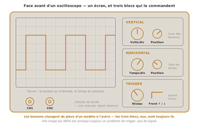
The oscilloscope displays voltage as a function of time: where the multimeter gives a value, the oscilloscope shows a waveform — the signal’s evolution, instant by instant. It is the indispensable instrument as soon as a signal changes fast: visualising a PWM, measuring a frequency and a duty cycle, spotting a button’s bounce, checking that a serial frame or a bus signal has the right shape. It only delivers with three settings properly understood — timebase, vertical scale and triggering (trigger). This page is a tool tutorial of the measuring instruments hub. For reading a waveform in itself, see timing diagram.

What is it for?

The oscilloscope answers questions the multimeter cannot handle:

• seeing the shape of a signal — square, sinusoidal, sawtooth, noisy — and not just its average value;
• measuring in time — the period and hence the frequency, the duty cycle of a PWM, a rise time, the duration of a pulse;
• spotting a dynamic fault — a bouncing contact, a parasitic oscillation, a signal collapsing under load, a glitch too brief for a multimeter;
• checking a communication — the shape of a UART, I²C or SPI frame (a logic analyzer decodes it, the oscilloscope shows its electrical quality).

For a simple DC value — a supply voltage, a resistance — the multimeter stays faster. The oscilloscope is reserved for signals that move.

Connecting the probe

The probe is the only link between the circuit and the screen. Connecting it properly is half the job:

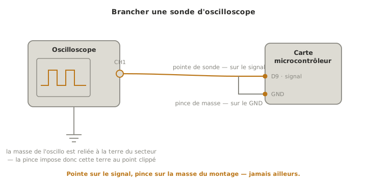
1. the probe cable screws onto a channel (CH1, CH2…) on the front panel;
2. at the other end, two contacts: the tip, which goes on the point to observe, and the ground alligator clip, which goes on the circuit ground — and nowhere else;
3. the why: through its power cord, the oscilloscope’s ground is tied to the mains earth. The clip therefore imposes earth on whatever point it touches — on the circuit ground, it establishes the common reference. On any other point, it creates a short circuit through the earth (see Pitfalls).

Getting started

1. Connect the probe as above — tip on the signal, clip on the circuit ground.
2. Set the vertical scale (Volts/div). The vertical axis is in volts: choose the scale so the signal fills a good part of the screen without overflowing.
3. Set the timebase (Time/div). The horizontal axis is in seconds: adjust it to see a few periods of the signal — neither a mush of squeezed oscillations, nor a single stretched period.
4. Set the trigger. This is the key setting: it tells the oscilloscope when to start tracing (for example “on the rising edge, when the signal crosses 1.6 V”). Without a correct trigger, the image scrolls and stays unreadable.
5. Account for the probe (×1 / ×10). A ×10 probe divides the signal by 10 — it allows measuring higher voltages without saturating, and loads the circuit less (cf. Measuring is not neutral, at the hub): the oscilloscope must be set to ×10 to display the true value.
6. Read amplitudes and durations on the grid, or through the meter’s automatic measurements.

Note

The trigger turns a scrolling signal into a stable image. A periodic signal retraced without synchronisation “slides” across the screen. The trigger sets a common starting point for every sweep (an edge, a level): the traces stack up and the signal looks frozen, hence readable. An unstable signal on screen is almost always a trigger problem, not a signal problem.

Example — Watching a PWM signal

The goal is to check the signal produced by an analogWrite() on an Arduino board: its shape, its frequency and its duty cycle.

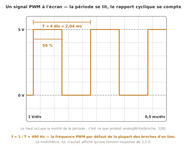
1. Connect the probe tip on the PWM pin, the ground clip on the board’s GND.
2. Set the vertical scale around 1 to 2 V/div (0–5 V signal) and the timebase to see a few periods.
3. Trigger on the rising edge, level ≈ 2.5 V: the square signal freezes.
4. Read the frequency: measure the period T on the horizontal axis. The frequency is 1/T (≈ 490 Hz on most Arduino PWM pins by default).
5. Read the duty cycle: the share of time spent high over one period. An analogWrite(broche, 128) command (half of 255) should give ≈ 50%, a command of 64 ≈ 25%.

You have confirmed not only that the signal comes out, but at what frequency and with what duty cycle — information the multimeter, which would only have shown an average voltage, could not give.

Pitfalls

Forgetting the common ground — short circuit through the earth. The ground of a bench oscilloscope is tied to the mains earth. Clipping the ground clip onto a point that is not the circuit ground ties that point to earth: short circuit, possible damage. Always connect the ground clip to the circuit ground, and be doubly careful on a circuit connected to the mains.

Undeclared ×10 probe. If the probe is in the ×10 position but the oscilloscope set to ×1, all the amplitudes read are wrong, by a factor of 10. Check the probe / setting agreement before measuring.

Wrong trigger. A trigger level outside the signal’s range, or the wrong edge, leaves the image scrolling. Set the level within the signal’s real amplitude.

Unsuitable timebase. Too fast, you only see a piece of the period. Too slow, the signal squeezes into a line. Adjust it for a few periods on screen.

Mixing up the amplitudes. Peak, peak-to-peak (Vpp) and RMS describe different quantities: read the right one for what you are after (see timing diagram).

Underestimating the bandwidth. An oscilloscope and its probe have a maximum bandwidth: a signal too fast comes out rounded or attenuated. For the slow signals of a student project this is rarely limiting, but keep it in mind on very steep edges.

See also

• Measuring instruments — the hub: method and choice of instrument
• Multimeter — when a single value is enough
• Function generator (GBF) — the natural pair: inject on one side, watch on the other
• Timing diagram — reading and interpreting a waveform (conceptual prerequisite)
• Electronic simulation — the simulated curve, the expectation to compare the real trace with
• PWM — the square signal most often watched on an oscilloscope
• Reading a datasheet — the characteristics (levels, timings) to check