The function generator (in French labs usually called the GBF, for générateur basse fréquence, low-frequency generator) is the reverse instrument of measurement: instead of reading what the circuit does, it injects a calibrated signal into it (sine, square, triangle) whose shape, frequency and amplitude you choose. It lets you test a circuit with a perfectly known input, without waiting for the real signal — sensor, microcontroller — to be available. This is a tool tutorial of the measuring instruments hub.
What is it for?
Testing a circuit requires an input. As long as the sensor is not wired or the program is not written, that input does not exist. The GBF creates it:
- stimulate a sub-assembly with a controlled signal: you know exactly what goes in, you watch what comes out on the oscilloscope — the response is compared with an expected one;
- temporarily replace a missing element: simulating the output of an analog sensor to test the conditioning stage or an ADC input before the real sensor arrives;
- characterise: sweeping several frequencies to plot a filter’s response, raising the amplitude to find the threshold of an input.
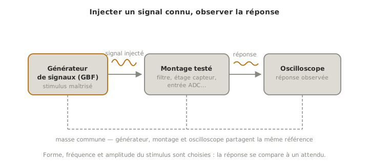
The GBF and the oscilloscope work as a pair: one injects, the other watches. It is the bench version of the simulation / measurement duo, except that here everything is real.
Essential settings
Four parameters define the signal:
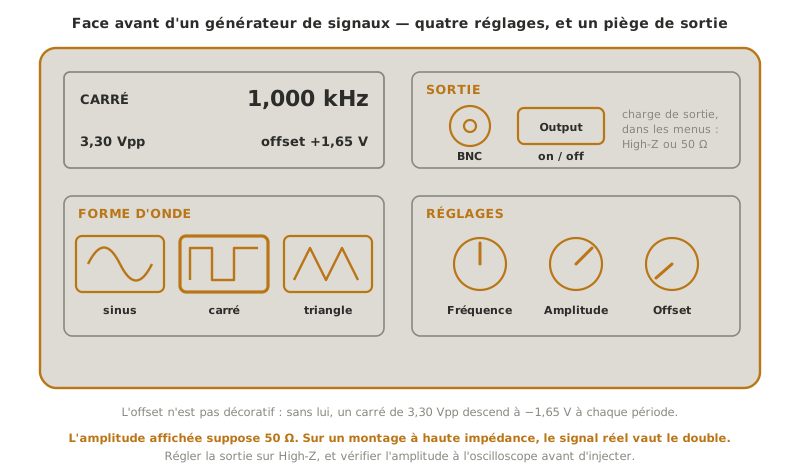
- the waveform — sine (frequency response, “analog” signals), square (logic signals, clocks, PWM testing), triangle (ramps, threshold tests);
- the frequency — that of the phenomenon to reproduce;
- the amplitude — watch the displayed unit: peak-to-peak (Vpp) most of the time;
- the offset — the DC shift of the signal. It is what turns a signal centred on zero into a purely positive one: for a 3.3 V logic input, set a 3.3 Vpp square with a +1.65 V offset — never a negative voltage on a microcontroller pin → logic levels.
The classic trap: High-Z or 50 Ω
The generator computes the displayed amplitude assuming a 50 Ω load on its output. Connected to a high-impedance input (an ordinary electronic circuit), the real signal is twice the displayed value. Before any injection: set the output to High-Z in the menus (or mentally divide by two), and check the real amplitude on the oscilloscope.
Connect and inject
- Set before connecting: shape, frequency, amplitude, offset — output disabled.
- Check the signal on the oscilloscope alone, before injecting it into the circuit: real amplitude, real offset.
- Connect the grounds: the shield of the BNC cable carries the generator’s ground, to be joined to the ground of the circuit.
- Inject and watch the response — keeping amplitude and offset within the range the circuit tolerates.
Pitfalls
Trusting the displayed amplitude. The High-Z / 50 Ω setting (see the warning) is the first cause of “I send 3.3 V, it receives 6.6”. Systematic check on the oscilloscope.
Injecting negative voltage into a logic input. A sine or a square without offset goes below 0 V on every period: a microcontroller input does not survive that for long. The offset is not a decorative setting.
Exceeding what the circuit tolerates. The amplitude is chosen from the circuit under test (its datasheet, its levels), not from what the generator can produce.
Forgetting the common ground. Without a shared reference, the injected signal means nothing to the circuit — and neither does the measurement at the output.
Where it fits in the project
- Proof of concept phase — testing one stage of the chain without waiting for the others: the processing chain is validated with a synthetic signal before the real sensor is connected.
- Integration and testing phase — producing repeatable test cases: the same ramp, the same square, on every run, which a real sensor never guarantees.
See also
- Measuring instruments — the hub: common method and choice of instrument
- Oscilloscope — the natural teammate: inject on one side, watch on the other
- ADC — the analog input most often tested with a GBF
- Logic levels — the range to respect before injecting anything