PID control in MicroPython

A PID (Proportional-Integral-Derivative) is a controller that continuously adjusts a command to bring a measured quantity towards a setpoint: it works out the error (setpoint − measurement) and derives from it a command combining three terms. It is the reference tool of closed-loop control — controlling a speed, a temperature, a position. Putting it to work rests on a calculation repeated at a constant time step, so on a steady rate through ticks_ms(). The algorithm is the same as in C++. Only the syntax changes.

What is it for?

Commanding “blind” is not enough as soon as you are aiming at a precise quantity in the face of disturbances. Putting a fixed PWM on a motor does not guarantee its speed: under load, it slows down. The closed loop measures the result, compares it to the setpoint, and corrects without stopping. The PID combines three behaviours: P is proportional to the current error: reactive, but it leaves a residual error. I accumulates the past error: it removes the residual, at the risk of winding up. D reacts to the rate of change: it damps, but it amplifies noise.

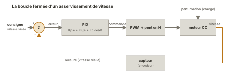
Block diagram of the closed loop: the setpoint enters a comparator (error = setpoint − measurement), the PID derives from it a command sent as PWM to the H-bridge that drives the motor; a sensor (an encoder) measures the real speed and sends it back to the comparator; a disturbance (the load) acts on the motor.|680

You put it in place in proof of concept, as soon as a function has to hold a setpoint despite the disturbances.

Step by step

Four steps: define the error, code the three terms, pace it at a constant step, tune the gains.

1. Define setpoint, measurement and error

consigne = 30000          # e.g. target speed (sensor unit, read_u16)
mesure = 0
erreur = consigne - mesure

2. Code the three terms

You keep the previous error and the accumulation between two steps. As Python has no constrain, a small borne() clamps a value:

Kp, Ki, Kd = 1.8, 0.6, 0.05      # gains to tune
integrale = 0.0
erreur_prec = 0.0
 
def borne(x, lo, hi):
    return max(lo, min(hi, x))
 
def calculer_pid(erreur, dt):
    global integrale, erreur_prec
    integrale += erreur * dt                       # term I: accumulate
    integrale = borne(integrale, -50000, 50000)    # anti-windup
    derivee = (erreur - erreur_prec) / dt          # term D: rate of change
    erreur_prec = erreur
    return Kp * erreur + Ki * integrale + Kd * derivee

3. Pace the calculation at a constant step

The I and D terms only make sense if dt is constant. You run the calculation at a fixed rate with [[micropython-temporisation-en|ticks_ms()]] (or, for something precise, a timer), and you clamp the command to the actuator’s range (duty_u16: 0-65535):

from machine import Pin, PWM
from time import ticks_ms, ticks_diff
 
moteur = PWM(Pin(15)); moteur.freq(1000)
DT_MS = 20
t_calc = ticks_ms()
 
while True:
    if ticks_diff(ticks_ms(), t_calc) >= DT_MS:
        t_calc = ticks_ms()
        erreur = consigne - lire_vitesse()
        commande = calculer_pid(erreur, DT_MS / 1000)
        moteur.duty_u16(int(borne(commande, 0, 65535)))

4. Tune the gains (Kp, Ki, Kd)

Tuning is empirical, in this order: start from Ki = Kd = 0, raise Kp until the response is fast and starts to oscillate, then back it off a little; bring Ki up to wipe out the residual error without reintroducing a slow oscillation. Finally, add Kd sparingly to damp, stopping as soon as the noise gets in the way. Watching measurement and setpoint over time guides you far better than trial and error.

Take a screenshot of Thonny’s plotter (Traceur) showing two curves, the constant setpoint and the measurement converging towards it.

Example — Controlling the speed of a motor

The speed of a DC motor is put under control: a sensor gives the real speed, the PID adjusts the PWM of the H-bridge to stick to the setpoint, even under load.

from machine import Pin, PWM
from time import ticks_ms, ticks_diff
 
moteur = PWM(Pin(15)); moteur.freq(1000)
 
consigne = 30000
Kp, Ki, Kd = 1.8, 0.6, 0.05
integrale = 0.0
erreur_prec = 0.0
DT_MS = 20
t_calc = ticks_ms()
 
def borne(x, lo, hi):
    return max(lo, min(hi, x))
 
def lire_vitesse():
    ...                       # supplied by the sensor (encoder, tachometer)
 
while True:
    if ticks_diff(ticks_ms(), t_calc) >= DT_MS:
        t_calc = ticks_ms()
        dt = DT_MS / 1000
 
        mesure = lire_vitesse()
        erreur = consigne - mesure
 
        integrale += erreur * dt
        integrale = borne(integrale, -50000, 50000)   # anti-windup
        derivee = (erreur - erreur_prec) / dt
        erreur_prec = erreur
 
        commande = Kp * erreur + Ki * integrale + Kd * derivee
        moteur.duty_u16(int(borne(commande, 0, 65535)))
 
        print(consigne, mesure)                       # for the plotter

How to read this code

On every step (every 20 ms), the block runs through the three terms. erreur = consigne − mesure: the gap to correct. integrale += erreur * dt accumulates the error over time (term I), immediately clamped by borne(…, -50000, 50000). That is the anti-windup. derivee = (erreur − erreur_prec) / dt measures the rate of change of the error (term D), then erreur_prec is stored for the next step. The command is the weighted sum Kp*erreur + Ki*integrale + Kd*derivee, and finally borne(…, 0, 65535) brings it back into the duty_u16 range before driving the motor. The two printed values (setpoint and measurement) are what you use to tune the gains by eye on the plotter.

The borne on the integral is the anti-windup: without it, if the actuator saturates (PWM already at maximum but the setpoint out of reach), the integral swells and the command takes a long time to come back down when the error reverses. The setpoint and measurement pair printed out feeds the plotter, to tune the gains by eye.

Pitfalls

Computing the PID at an irregular step. The I and D terms depend on dt. A calculation done sometimes every 5 ms, sometimes every 50 ms, falsifies the integral and the derivative. Pacing it at a fixed interval ([[micropython-temporisation-en|ticks_ms()]] or a timer) is not negotiable.

Forgetting the anti-windup. When the actuator saturates, the integral accumulates into the void. At the reversal of the error, the command stays “stuck” for far too long. Clamp the integral (or the command).

Too much derivative on a noisy signal. The D term amplifies noise: a noisy sensor plus a high Kd gives a command that shakes. Filter the measurement (a moving average) or reduce Kd.

Not clamping the command. The PID output can go beyond 0-65535: int() on an out-of-range value raises an error or produces wrong behaviour. Always borne() before duty_u16.

Forgetting global in the calculation. integrale and erreur_prec have to be declared global (or carried by an object or a class), otherwise they start again from zero on every call.

Believing a PID makes up for a faulty rig. A badly placed sensor, an undersized actuator, mechanics that bind: no gain corrects a hardware defect.

Special case — A PID class, or a library

Wrapping the controller in a class (gains, integrale, erreur_prec as attributes, a calculer(mesure, dt) method) avoids the global statements and allows several independent PIDs (one per axis).
MicroPython PID libraries exist (installable through mip, see libraries) and handle time step, anti-windup and clamping. Handy in production. Doing the maths by hand stays preferable in order to understand before delegating.

Where it fits in the project

Steps 2-3 of the proof of concept phase — validating the control of a function (speed, position, temperature) on an isolated rig, with the real sensor and actuator.
Integration and testing phase — the control loop runs at the constant step imposed by a timer. Its gains, tuned during the proof of concept, are checked again on the complete system and under load.

A PID is designed around a reliable measurement and a steady rate: those two prerequisites count as much as the gains.

TheSkillCodex

Explorateur