PID control on Arduino

A PID (Proportional-Integral-Derivative) is a controller that continuously adjusts a command to bring a measured quantity to a setpoint: it computes the error (setpoint − measurement) and derives from it a command combining three terms. It is the reference tool of closed-loop control (controlling a speed, a temperature, a position) and running one on an Arduino rests on a calculation repeated at a constant time step, so on steady timing.

What is it for?

Driving something “blind” is not enough as soon as you aim at a precise quantity in the face of disturbances. Putting a fixed voltage on a motor does not guarantee its speed: under load, it slows down. The principle of the closed loop is to measure the result, compare it with the setpoint, and correct the command accordingly, over and over. PID is the most widespread correction law because it combines three complementary behaviours:

• P (proportional) — corrects in proportion to the current error: quick to react, but often leaves a steady-state error;
• I (integral) — accumulates past error: removes the steady-state error, at the risk of winding up;
• D (derivative) — reacts to the rate of change of the error: damps and anticipates, but amplifies noise.

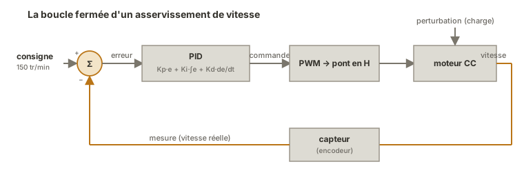
You put a PID in place during the proof of concept, as soon as a function has to hold a setpoint despite disturbances, typically speed or position control.

Step by step

Four steps: measure and compute the error, code the three terms, run the calculation at a fixed rate, then tune the gains.

1. Define setpoint, measurement and error

The loop needs three quantities: the setpoint (what you want), the measurement (what you have, from a sensor), and the output command (to the actuator, often a PWM signal). The error is their difference.

double consigne = 150.0;   // e.g. target speed (rpm)
double mesure   = 0.0;     // read from a sensor
double erreur   = consigne - mesure;

2. Code the three terms

The calculation combines the current error (P), its accumulation (I) and its rate of change (D). You keep the previous error and the accumulation between two steps.

double Kp = 2.0, Ki = 0.5, Kd = 0.1;   // gains to tune
double integrale = 0, erreurPrec = 0;
 
double calculerPID(double erreur, double dt) {
  integrale += erreur * dt;                       // I term: accumulate
  double derivee = (erreur - erreurPrec) / dt;    // D term: rate of change
  erreurPrec = erreur;
  return Kp * erreur + Ki * integrale + Kd * derivee;
}

3. Run the calculation at a constant step

A PID assumes a regular calculation interval dt: the I and D terms only mean something if the step is constant. So you run the calculation at a fixed rate, with [[arduino-temporisation-en|millis()]] or, where precision matters, a hardware timer. The result drives the actuator, clamped to the usable range of the command.

const unsigned long DT_MS = 20;        // 20 ms step (50 Hz)
unsigned long tCalcul = 0;
 
void loop() {
  if (millis() - tCalcul >= DT_MS) {
    tCalcul += DT_MS;                              // step the date on, never read it back
    double erreur = consigne - lireVitesse();
    double commande = calculerPID(erreur, DT_MS / 1000.0);
    commande = constrain(commande, 0, 255);        // PWM clamp
    analogWrite(MOTEUR, (int)commande);
  }
}

4. Tune the gains (Kp, Ki, Kd)

Tuning is empirical and goes in this order:

• start from Ki = Kd = 0, raise Kp until the response is fast and starts to oscillate, then back off a little;
• bring Ki up gradually to make the steady-state error disappear, without bringing back a slow oscillation;
• add Kd sparingly to damp overshoot, stopping as soon as noise becomes a nuisance.

Watching the measurement and the setpoint over time guides this tuning far better than blind trial and error.

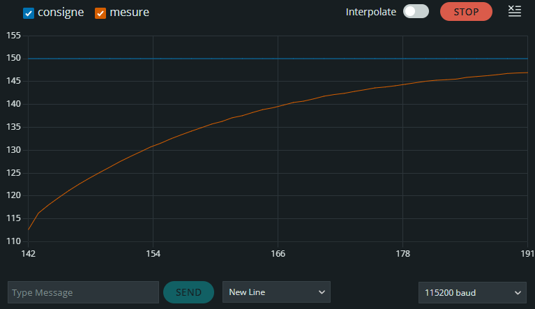
The curve above comes from a simulated process (a motor model computed inside the sketch itself, with no motor and no sensor) and it reads in two stages. The measurement jumps from 0 to more than 110 rpm in two tenths of a second, because the initial error saturates the command at 255, and that is the P term at work. Then it ramps towards the setpoint over about ten seconds, and this second stage belongs to the I term, which closes the steady-state error all the more slowly as Ki is small. A trace that seems to stall below the setpoint is therefore not a broken loop, it is a cautious Ki.

Reproducing this curve without a motor. The Example below declares double lireVitesse(); without ever defining it: the sensor is assumed to be supplied, so the sketch does not link as it stands. The block below replaces it with a first-order motor model computed in software. The speed tends towards GAIN_MOTEUR × commande with a time constant TAU_S. A board and a USB cable are enough, there is nothing to wire.

// Simulated process: replaces the `double lireVitesse();` line of the Example
 
const double GAIN_MOTEUR = 1.5;   // rpm per PWM unit (255 gives 382 rpm)
const double TAU_S       = 0.30;  // mechanical time constant, in seconds
double vitesseSimulee    = 0.0;   // model state: the "real" speed
 
double lireVitesse() {            // stands in for the sensor: returns the model state
  return vitesseSimulee;
}
 
void simulerMoteur(int commande, double dt) {   // advances the model by one step
  vitesseSimulee += dt / TAU_S * (GAIN_MOTEUR * commande - vitesseSimulee);
}

Then two insertions into the loop of the Example. First make the process react to the command, right after analogWrite (without this line the model stays still and the measurement never moves):

    simulerMoteur((int)commande, dt);   // the process reacts to the command

Then replace the printing with the form below. The labels name the two curves in the plotter legend and stay in French, so that they read the same as the screenshot above. Spacing matters too: at 50 lines a second, the plotter window only holds one second of history, and convergence is invisible in it.

    static byte n = 0;
    if (++n >= 10) {                    // one line in ten, so 5 points a second
      n = 0;
      Serial.print("consigne:"); Serial.print(consigne);
      Serial.print(" mesure:");  Serial.println(mesure);
    }

The model gain is not arbitrary: with the integral clamped at 200, the I term on its own can only carry a command of Ki × 200, that is 120. A simulated motor that is too weak would need more in steady state, and the loop would settle below the setpoint (see Pitfalls).

Example — controlling the speed of a DC motor

You control the speed of a DC motor in closed loop: a sensor (encoder, tachometer) gives the real speed, the PID adjusts the PWM sent to the H-bridge to stick to the setpoint, even when the load varies.

const int MOTEUR = 9;          // PWM command to the H-bridge
 
double consigne = 150.0;       // target rpm
double Kp = 1.8, Ki = 0.6, Kd = 0.05;
double integrale = 0, erreurPrec = 0;
 
const unsigned long DT_MS = 20;
unsigned long tCalcul = 0;
 
double lireVitesse();          // supplied by the sensor (encoder, etc.)
 
void setup() {
  pinMode(MOTEUR, OUTPUT);
  Serial.begin(115200);
}
 
void loop() {
  if (millis() - tCalcul >= DT_MS) {
    tCalcul += DT_MS;                                // strictly constant rate
    double dt = DT_MS / 1000.0;
 
    double mesure = lireVitesse();
    double erreur = consigne - mesure;
 
    integrale += erreur * dt;
    integrale = constrain(integrale, -200, 200);     // anti-windup
    double derivee = (erreur - erreurPrec) / dt;
    erreurPrec = erreur;
 
    double commande = Kp * erreur + Ki * integrale + Kd * derivee;
    commande = constrain(commande, 0, 255);
    analogWrite(MOTEUR, (int)commande);
 
    Serial.print(consigne); Serial.print(' '); Serial.println(mesure);
  }
}

How to read this code

At each step (every 20 ms), the block runs through the three terms. erreur = consigne − mesure: the gap to correct. integrale += erreur * dt accumulates the error over time (I term), immediately clamped by constrain. That is the anti-windup. derivee = (erreur − erreurPrec) / dt measures the rate of change of the error (D term), then erreurPrec is stored for the next step. The command is the weighted sum Kp·erreur + Ki·integrale + Kd·derivee, and finally constrain(…, 0, 255) brings it back into the PWM range before analogWrite. The two printed values (setpoint and measurement) are what you use to tune the gains by eye on the serial plotter.

The constrain on the integral is an anti-windup clamp: without it, if the motor saturates (PWM already at 255 but the setpoint out of reach), the integral grows without bound and the command takes a long time to “come back down” when the error reverses. Clamping the integral avoids that overshoot. The setpoint and measurement being printed together feed the serial plotter for tuning the gains by eye.

Pitfalls

Computing the PID at an irregular rate. The I and D terms depend on dt. A calculation called sometimes every 5 ms, sometimes every 50 ms, distorts the integral and the derivative. Running the calculation at a fixed interval ([[arduino-temporisation-en|millis()]] or a timer) is not negotiable.

Forgetting the anti-windup clamp. When the actuator saturates, the integral keeps accumulating into nothing: when the error reverses, the command stays “stuck” for too long. Clamping the integral (or the command) fixes this classic flaw.

Believing the anti-windup clamp has no effect in steady state. An integral clamped at ±200 only lets the I term carry a command of Ki × 200. If the working point you aim at needs more (a weak motor, a heavy load), the integral sits on its clamp and the loop settles with a steady-state error, with nothing to signal it. The clamp is sized on the command actually needed, not on a round number.

Putting too much derivative on a noisy signal. The D term amplifies measurement noise: a noisy sensor plus a high Kd gives a command that shakes. Filter the measurement or reduce Kd.

Not clamping the command. The PID output can go beyond the actuator range (PWM 0-255). Without constrain, the value is truncated any old how. Always clamp explicitly.

Believing a PID makes up for a faulty setup. A badly placed sensor, an undersized actuator or a mechanism that binds are not fixed with gains. A PID corrects a command, not a hardware fault.

Tuning the three gains at once. You can no longer see what each one does. The approach is sequential: Kp, then Ki, then Kd.

Special case — the PID_v1 library

Rather than coding the calculation by hand, the PID library (Brett Beauregard, PID_v1) provides a ready-made controller that handles the time step, the anti-windup clamp and the limits. You pass it references to the input, the output and the setpoint, plus the gains, then you call Compute() at regular intervals. It also computes the derivative on the measurement rather than on the error, which avoids the “derivative kick” (a sudden spike in the command) when the setpoint changes abruptly, a refinement the hand-written calculation above does not include. Handy in production. The hand-written calculation stays preferable for understanding what the library does, before letting it do the work.

Where it fits in the project

• Steps 2-3 of the proof-of-concept phase — validating the closed-loop control of a function (speed, position, temperature) on an isolated bench, with a real sensor and a real actuator, before integration.
• Integration and testing phase — the control loop runs at the constant step imposed by a timer. Its gains, tuned during the proof of concept, are checked again on the complete system and under load.

A PID is designed around a reliable measurement and a steady rate: these two prerequisites (sensor, time base) count as much as the gains themselves.

See also

• Closed-loop control — the parent concept: closed loop, setpoint, error and controller, the role of the PID
• delay() vs millis() — running the calculation at a constant step
• Hardware timers — for a precise time step on a demanding control loop
• Driving a PWM output — the output command of the controller
• DC motor — the actuator of the example (H-bridge)
• Reading an analog sensor — the measurement that closes the loop
• Non-blocking programming — the PID is one timed task among others
• Arduino — hub for the Arduino tutorials