Closed-loop control is a command that never stops checking itself: instead of driving a system “blind”, you measure the quantity being regulated, compare it with the setpoint (the target value) and correct the command from the error (setpoint − measurement), continuously. That permanent return of the measurement is what separates closed-loop control from open-loop command, and what lets it hold a setpoint despite disturbances.
What is it for?
In open loop, you apply a command without checking the result: putting a fixed voltage on a motor means hoping for a speed. But under load it slows down, and nothing catches it. As soon as you aim at a precise quantity in the face of unknowns (load, temperature, friction, ageing), open loop is no longer enough.
Closed loop turns the logic around: it watches the gap to the setpoint continuously and acts to reduce it. That is what makes it possible to regulate a speed, a position, a temperature or a level with an accuracy that no longer depends on the quality of the model, but on the quality of the measurement and of the correction. The price to pay: you need a sensor, a regular computing rate, and careful tuning: a badly tuned control loop oscillates or diverges where open loop merely stayed imprecise.
How does it work?
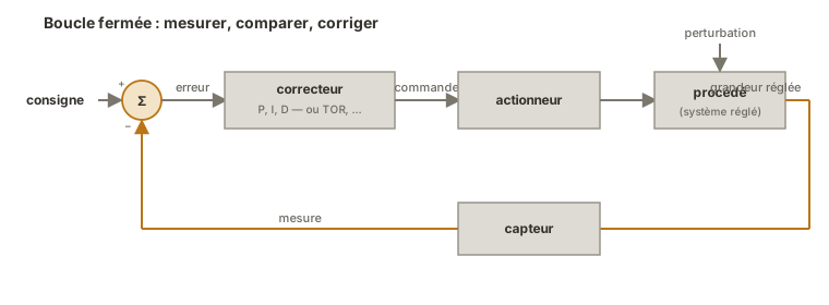
Four elements make up the loop.
- The comparator and the error. A summing point permanently computes the error = setpoint − measurement. It is the driving signal of the whole control system: as long as it is not zero, the system has a reason to act.
- The controller. It turns the error into a command. Its law can be simple (the on-off of a thermostat) or continuous. The most widespread is the PID, which combines three reactions to the error (see below).
- The actuator and the process. The command goes through an actuator (a motor via a PWM, a heating resistor…) that acts on the process — the physical system whose quantity you are regulating. That is also where disturbances get in.
- Feedback from the sensor. A sensor measures the regulated quantity and closes the loop by bringing it back to the comparator. The whole control system hangs on that measurement: a noisy, slow or badly placed sensor caps the quality of the regulation, whatever the tuning.
On top of that comes a constraint of digital implementation: the computation repeats at a constant time step (→ timer), otherwise the terms that depend on time lose their meaning.
The PID controller
The PID (Proportional-Integral-Derivative) sums three terms, each reacting differently to the error:
- P — proportional to the current error: responsive, but often leaves a residual error;
- I — proportional to the accumulated error: cancels the residual error, at the risk of winding up if the actuator saturates;
- D — proportional to the rate of change of the error: damps and anticipates overshoot, but amplifies noise.
Tuning a PID means arbitrating between speed, stability and accuracy: too much gain and the system oscillates. Too little and it responds sluggishly. Tuning is empirical and sequential (P, then I, then D), guided by watching the response over time.
Pitfalls
Closing the loop where open loop would do. If the quantity is stable and the disturbances are negligible, a direct command (properly calibrated) is simpler and more robust. Closed loop has a cost — sensor, tuning, risk of instability — that has to be justified.
Raising the gains until it goes unstable. Too strong a gain makes the loop oscillate, or even diverge: the system chases the setpoint and overshoots it more and more. Stability comes before speed.
Neglecting the sensor. Regulation can never be better than its measurement: a noisy sensor makes the command shake, a slow sensor introduces a destabilising delay. The weak link of a control loop is often the feedback path, not the controller. Filtering the measurement attenuates the noise, but adds a delay that can destabilise the loop in its turn.
Forgetting actuator saturation. When the actuator is flat out but the setpoint is still out of reach, the integral term keeps accumulating into the void (wind-up): when the error reverses, the command takes a long time to come back down. The cure is to clamp the integral (anti-windup).
Believing that good tuning makes up for a bad build. Gains compensate neither an undersized actuator, nor a mechanism that binds, nor a badly placed sensor. Control tunes a command, not a hardware defect.
See also
- Open loop — command without measurement, and the four conditions that make it legitimate
- PID control on Arduino — the PID controller put to work
- PID control in MicroPython — the same loop, written in MicroPython
- Functional block diagram — the formalism of blocks and flows of which the closed loop is one case
- PWM — the typical way a microcontroller commands an actuator
- Driving a DC motor on Arduino — the most common controlled actuator in a project
- Driving a DC motor in MicroPython — the same actuator, driven from MicroPython
- Reading an analog sensor on Arduino — the feedback that closes the loop
- Reading an analog sensor in MicroPython — the same reading, on the MicroPython side
- Filtering measurements — cleaning up the feedback without adding a delay that destabilises it
- Timer — the time base that paces the computation at a constant step