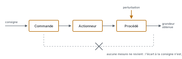
An open-loop command applies an action without measuring its result: you send the command, and you trust the build to produce the expected effect. It is the command mode of the vast majority of systems (a heater on a timer, a stepper turned by a number of steps, an LED you switch on). So the useful question is not “do we need closed-loop control?” but the opposite: under what conditions can we do without measuring?
What is it for?
Open loop is not a fallback: it is the default choice, and it is often the right one. It needs no sensor, so no extra wiring, no conversion, no filtering, no computing rate to hold. It cannot oscillate (the failure that lies in wait for every badly tuned control loop). And it is debugged by looking at a single chain, from top to bottom, without wondering whether the symptom comes from the measurement or from the correction.
The price is unique and it is total: the system does not know what it is doing. Any gap between the intended effect and the effect obtained — due to a load, to wear, to a temperature, to a fault — stays invisible and uncorrected. The whole question therefore lies in an honest assessment of those gaps.
The four conditions
An open-loop command holds if all four of the following conditions are met. It only takes one to fail for measurement to become necessary again.
- The behaviour is predictable. You know, by calculation or by a trial, which command produces which effect. A stepper advances by a known angle per step. A heating resistor warms up reproducibly in a given volume.
- Disturbances stay bounded. They always exist, but their cumulative effect must stay within the tolerance allowed. That is a comparison in figures, not an impression: if the requirements ask for ± 0.5° and the load costs 2°, the condition is violated.
- The origin is known. A relative command (“advance by 30°”) is only worth something if you know where you started. Hence the homing move at start-up, against an end stop or a limit switch: a single measurement point, once, which is not a closed loop.
- There is no cumulative drift. An error that adds to the previous one always ends up exceeding the tolerance, however tiny it is. It is the condition most often overlooked, and the one that tips over a system that looks healthy (see Special case).
Example — the 3-axis arm, open loop and not quite
The three axes of the arm are driven by steppers, with no position feedback: the program counts the steps, and the angle follows. The four conditions are examined one by one: the behaviour is predictable (known angle per step), the forces are bounded by the sizing, the origin is taken at start-up against the limit switches, and the fourth condition is the worrying one.
That is why the arm still carries three angle sensors: not to correct continuously, but to watch the gap between the commanded position and the real one. So the build is neither pure open loop nor closed-loop control: it measures to detect, not to correct.
It is a very common configuration on a project, and it deserves a name: open-loop command with monitoring. It costs the sensor but not the tuning, and it turns a silent failure into a reported fault.
Pitfalls
Confusing “it worked in the trial” with “the conditions are met”. A trial that succeeded unloaded, cold, on a brand-new unit says nothing about disturbances in service. The four conditions are assessed on the worst case of use, not on the demonstration.
Forgetting the homing move. A system with relative commands that starts up assuming it is at zero is wrong by everything that has moved since power-off, including by hand, including under its own weight. The origin is taken at every power-up, never once and for all.
Taking repeatability for trueness. An open-loop command can be remarkably repeatable (returning always to the same place) and yet systematically wrong by a few degrees. With no measurement, nothing tells the two apart, and only an external check reveals it (see accuracy of measurement).
Compensating a drift with a hard-coded correction. Adding “+3 steps every ten turns” because a loss was observed means modelling a defect instead of fixing it. The correction holds for today’s load and lies for every other one.
Switching to closed loop at the first gap. The opposite is just as real a trap. Closing the loop brings a sensor, a rate to hold, gains to tune and a risk of oscillation. Before going there, check which of the four conditions has failed: often it is the mechanics or the sizing that needs revisiting, not the command.
Special case — the lost step
The stepper is the canonical example of open loop, and it also carries its signature failure. When the torque demanded exceeds what the motor can deliver — too sharp an acceleration, an obstacle, undersizing —, the rotor does not follow the pulse: the step is lost. Nothing reports it. The program, for its part, keeps counting as if nothing had happened.
The gap between the real position and the assumed one is then permanent and cumulative: every lost step adds to the previous one until the next homing move. An arm that slowly drifts over the cycles does not have a program problem, it has lost steps.
It is exactly the fourth condition that fails, and the cure is chosen in this order: reduce the acceleration, increase the torque margin, and only then add a measurement (monitoring the gap if you want to detect, closed-loop control if you want to correct).
See also
- Closed-loop control — the closed loop, when one of the four conditions fails
- Functional block diagram — the formalism where the presence or absence of feedback is read at a glance
- Energy chain — the command chain of which open loop is the form without feedback
- Choosing the hardware — the step where the choice of an actuator drivable in open loop is decided
- Accuracy, trueness, precision — repeatable is not true
- Driving a stepper (Arduino) and (MicroPython) — the canonical case put to work